Meta-learning and Monads

Meta-learning is an exciting approach to machine learning. Instead of training models to do particular tasks, it trains these models to learn how to do those tasks. Meta-learning is essentially learning squared: learning how to learn. There’s been plenty of exciting developments in this area, but in this blog post I want to explore one foundational aspect of it what it means to meta-learn.

Abstractly, a meta-learner is also a learner, one which has another learner nested inside of it. We might expect this meta-learner to satisfy a particular property: that these two levels of learners can be “collapsed” into just one big learner. Compare this with the concept of a monad in category theory and functional programming. A monad on some category has a property that for every object , there is a map called “join”. This map joins, or collapses down two levels of context to just one. For instance, if you’ve got the list monad, that means that you can collapse a list of lists down to just a list. In Haskell there is done with the map

which concatenates lists. It takes, say, [[1, 2],[4,5,6], [-37]] and produces [1,2,4,5,6,-37]. Or, if you’ve got the probability monad, then you can take a probability distribution on the space of probability distributions on some space and think of it just like a probability distribution on . That is, you collapse down two levels of probability distributions to one. Another example is the state monad. The join operation of the state monad tells us that two layers of stateful computation can be turned into just one layer of big stateful computation. And so on.

Thus a natural question to ask is: could meta-learning be formally interpreted as a monad? This is a deep question. Categorically formalising what “learning” is, even in the simplest case, is a daunting task. We would need a base category, an endofunctor on it which describes “learning”, and two operations: join and unit (I haven’t discussed the unit yet, but I will).

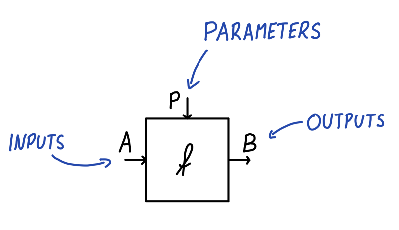
In our recent paper Categorical Foundations of Gradient-Based Learning we’ve got the construction Para which I believe is a first step. Given any symmetric monoidal category (throughout the post I’ll be thinking of the monoidal structure as Cartesian), we can form a category¹ which is defined as follows. It has the same objects as , but every morphism in isn’t just a morphism in . It’s a choice of some parameterising object and a map in . We think of as the inputs to a neural network, as the outputs and as the parameter space of the neural network, whose elements are usually called weights. Visualised below, the information flows from on the left to on the right, while being transformed by coming from above. I think of the parameters as the ship’s wheel, controlling the rudder down below and steering the flow of water from the inputs to the outputs. This means that for different choices of , via we get different implementations of a map of type . Abstractly, we can think of as a learner which is learning a map of type in . Our learning algorithm will search through the parameter space in order to find a such that the map is best, according to some criteria.

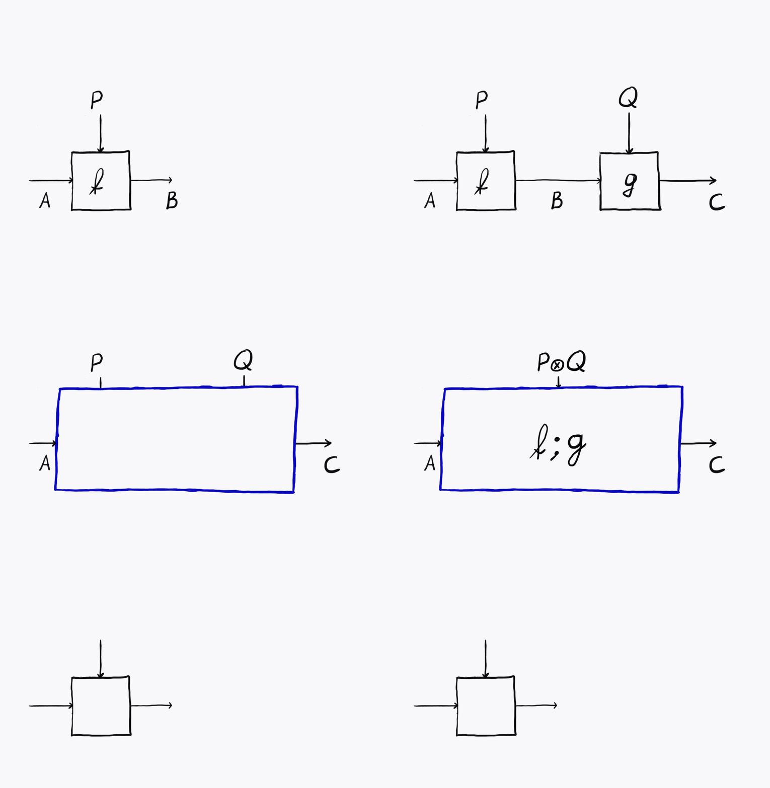
Parameterised maps can be composed. If you’ve got a -parameterised morphism and -parameterised , you can plug them together, obtaining a -parameterised morphism . This is visualised below.

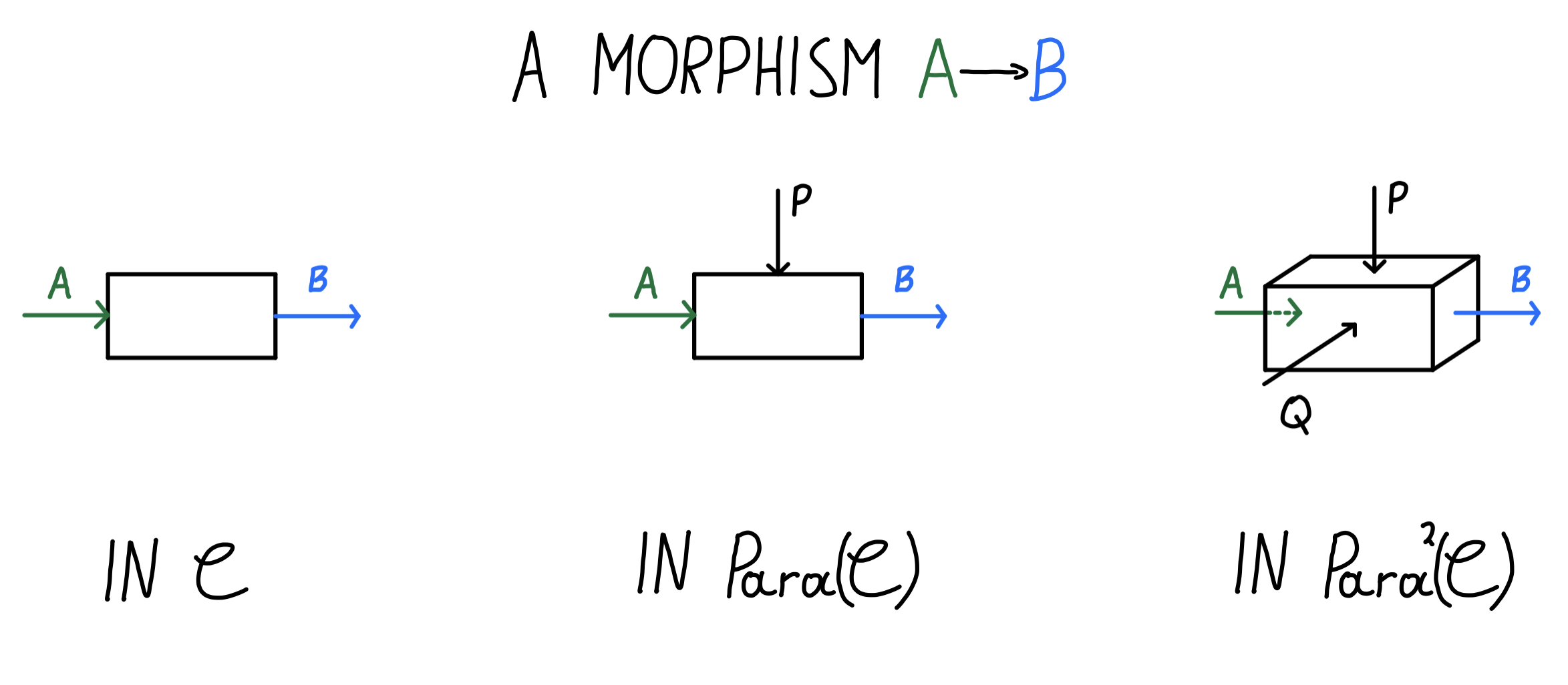
The category is useful because it allows us to state the fact that the parameter space of a neural network is more than just an object of the category: it’s part of the data of the morphism itself. There’s a lot more to say about this category, but what’s most interesting is that is itself a symmetric monoidal category. This allows us to apply to it again, yielding a category² with doubly-parameterised maps.

How do we think about these doubly-parameterised morphisms? Just as the path we took from thinking about maps in to maps in involved using an extra axis for the parameters, the same thing applies when we go from to (I’ll write for double Para from now on). A map in this category is a choice of some parameter object (which is just an object in ) and a morphism in . But a morphism in is itself a parameterised map! It involves a choice of an object and a map in . So we see that there were two levels of parameters to unpack. This can be neatly visualised below in three dimensions.

In fact, itself is an endofunctor, it’s type is , where the domain and codomain is the category of symmetric monoidal categories and symmetric monoidal functors.³ This means that can be applied not only to a symmetric monoidal category , but also to a functor between symmetric monoidal categories.

Finally, this brings us to the main idea of this blog post: is an endofunctor, but also more than that: it has the structure of a monad.⁴ The join of this monad tells us that for every object in our category (and this object is now itself a symmetric monoidal category), there is a morphism (and this morphism is a symmetric monoidal functor) which takes any doubly-parameterised category and reinterprets it as a (singly-)parameterised category. The previously described morphism gets mapped to . Abstractly, it tells us that a -parameterised learner of a -parameterised learner of a map in can be reinterpreted of as a -parameterised learner of a map in in .

What about the unit of the monad? Let’s think about what should happen. The unit map of an arbitrary monad on assigns to each object a map . We think of it as taking something outside of any context and putting it in a trivial context. For the list monad, it takes any element a and puts it in a list containing just that one element a. In Haskell, this is done with the map return : a -> [a] which takes, say, an integer 3 and maps it to the list [3]. Similar story happens with the probability monad. Any element can be interpreted as a “deterministic” probability distribution using the dirac delta at . For the state monad, the unit takes an element and wraps in on a context which independently of state always returns (and leaves the state unchanged).

What would we expect to happen for learners? Well, since somehow reinterprets the usually “unparameterised” category as parameterised, then we expect the unit to interpret an unparameterised morphism in as a parameterised one in . Which parametrised morphism is it? We first need to pick a parameter space. And the only object we can even refer to in an arbitrary monoidal category is the monoidal unit . Now we need to pick a morphism of type , and the natural choice is , where is the laxator of the monoidal category.

We didn’t do much, we just wrapped our morphism in some trivial context. This makes sense! If you look at the previous image, you can imagine that for the map in there’s a “secret”, but trivial input coming from the top. I’ve also drawn this explicitly below. This agrees with the idea of not drawing the wires of the monoidal unit.

So the unit of this monad tells us that any computation can be thought of as a trivially parameterised computation. In more abstract terms: for a system that doesn’t have some internal parameters and isn’t learning, we can say that it’s trivially learning. We can think of it as having a parameter space with only one element in it: you can always only pick that one parameter and there’s nothing to learn. And this is it: it’s easy to check that unit and join, as defined for , satisfy the monad laws.

Now, there’s still a big unanswered question: what part of this actually describes learning? We’ve only described what it means to be parameterised. This is true – is only a first step. However, this is also where we use the power of compositionality of category theory. By substituting the base monoidal category for the right category, we get very different things. As I’ve described in my other post, the category of learners is obtained when we set the base category to , the category of what I call “bidirectional maps”. These are maps which compute a forward value, but also receive a “gradient” which they propagate backwards.⁵ The interaction between and ends up propagating the right information to the right ports, which is quite astonishing.

But the story doesn’t end on a satisfying note. While optics allow us to talk about bidirectionality and parameter update, we need more. Learning is essentially about iteration: you do something, get feedback, update yourself and then go out into the world to try again. While some interesting things have been written about iteration of learning, no unifying categorical perspective has been given yet.

In more practical terms, this missing structure needs to account for two kinds of learning: standard learning where a learner is iterated, seeing different data-points as input at each time step, and meta-learning, where the meta-learner now sees as input whole iterations of learning at each time step. There is a lot of details here, and a number of different kinds of meta-learning can be found in the literature. The paper Learning to learn by gradient descent by gradient descent seems to be the closest to what I’m describing here.

There are many things left to understand. It’s hard to wrap our heads around what ought to happen when you’re learning to learn. We’re building a house, and it’s hard to do it without good foundations. Category theory provides a lot of steel beams, but it’s not clear how to use them just yet. Hopefully we can find a way and build skyscrapers people couldn’t have dreamt of a few hundred years ago.

Thanks to Ieva Čepaitė and Matteo Capucci for providing feedback on a draft of this post.